R. Mújica
INAOE-Tonantzintla, Mexico and
Observatoire Astronomique, Strasbourg, France
F.-J. Zickgraf
Observatoire Astronomique, Strasbourg, France
I. Appenzeller, J. Krautter
Landessternwarte-Heidelberg, Germany
A. Serrano
INAOE-Tonantzintla, Mexico
W. Voges
MPE-Garching, Germany
Introduction
A defining characteristic of BL Lac objectsis their lack of prominent
emission lines, indicative that their radiant energy is largely associated
with non-thermal processes. This feature has led to the fact that, BL Lac
objectshave been mainly identified for their radio or X-ray emission, with
the consequent subdivision of the class into radio-selected BL Lac objects
(RBLs) and X-ray-selected BL Lac objects(XBLs). Whether these two classes
correspond to different populations or to different aspects of the same
phenomenon is still in discussion. In general, they seem to exhibit different
properties, with RBLs being more core dominated, highly polarized, variable
and luminous at optical and radio wavelength than XBLs (see Perlman &
Stocke 1993; Jannuzi et al. 1994; Morris et al. 1991; Padovani 1992). It
also seems the two classes occupy different regions in the ![]() diagram, indicative of different energy distributions (Stocke et al. 1985;
Ledden & O'Dell 1985).
diagram, indicative of different energy distributions (Stocke et al. 1985;
Ledden & O'Dell 1985).
Extreme variability is among the most striking properties of BL Lac objectsand is therefore well suited as identification criterion. In general BL Lac objectsare variable across the electromagnetic spectrum, although there is a considerable range of variability properties, i.e. amplitudes, timescales, periodicity, etc. (Kollgard 1994).
During the identification program of a sample of ROSAT All-sky Survey
X-ray sources in the northern hemisphere (Zickgraf et al. 1997), the intrumentation
used did not permit to acquire spectroscopic data good enough to classify
the BL Lac objects in a reliable way. It was therefore neccesary to procede
in a different way. We monitored all the objects with a suspicious featureless
spectrum (from the ID project) and with a 4.85 GHz radio detection. In
addition, we computed the ![]() diagram
for the X-ray/radio sample in order to check the position of the candidates.
In this way, a variable object with a suspicious featureless spectrum and
adequate spectral indices can be reliable classified as a BL Lac.
diagram
for the X-ray/radio sample in order to check the position of the candidates.
In this way, a variable object with a suspicious featureless spectrum and
adequate spectral indices can be reliable classified as a BL Lac.
Here we present the results about the identification and the analysis
of the variability of the BL Lacs, we compare our method with other techniques
to identify BL Lacs, and also discuss the results with respect to the unification
models.
Selection of the sample
The original X-ray sample is described in Zickgraf et al. (1997). Six study areas north of were investigated. This complete, flux and area limited sample consists of 674 X-ray sources.
Based on the fact that there are no radio quiet BL Lac objects(Stocke et al. 1990), we crosscorrelated the sample with radio catalogues. We have selected those X-ray sources with a counterpart in the 87GB catalogue (Gregory & Condon 1991) or in the BWE Catalogue (Becker, White & Edwards 1991), both at a frequency of 4.85 GHz.
As the position uncertainty of both catalogues is , we selected only
the X-ray sources with a radio counterpart located closer than 120" from
the X-ray position. From this correlation we obtained 67 sources. This
is the X-ray/radio sample. We selected the objects with a suspicious featureless
spectrum and started to monitored them for optical variability.
Observations and Data Reduction
The observations were taken during seven runs with the 2.1m telescope of the Guillermo Haro Observatory in Cananea, Sonora, Mexico, and in the 1.23m telescope of the Calar Alto Observatory in Spain.
The data on the 2.1m telescope were collected with the Landessternwarte Faint Object Spectrograph and Camera (LFOSC). This instrument has a focal reducer that permits to obtain photometry and multi-object spectroscopy. It has a CCD with 22m pixel size as a detector and the field size is 10' X 6' (the scale is 1"/pix) (see Zickgraf et al. 1997). The 1.23m telescope was equipped with a TEK CCD and a Rc filter. The field size was 10' X 10'.
Each of the fields was observed, at least, once per night. The frames were reduced following a standard procedure (bias substraction, flat-field correction). In order carry out the differential photometry, we simulated aperture photometry in our frames. In addition to the BL Lac(s) candidate(s), we selected, at least, five non-saturated comparison stars of different brightness. The errors were estimated from the comparison stars with same brightness as the candidates.
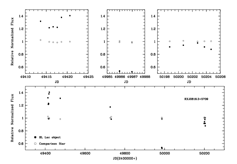
We computed the ratios of the countrates for each pair of objects and then we normalized them over all the data available. The variable comparison objects were rejected from the analysis. The final light curves were computed using one of the non-variable comparison stars as bright as the candidate and the check star was as bright or brighter than both (candidate and comparison). The errors are typically 1-3% and in the worst cases 5%. An example of a light curve is plotted in Figure 1.
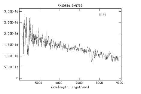
For the final list of candidates, additional data were obtained with
LFOSC (dispersion 360Å mm-1) in order to improved the
S/N ratio. As an example, the spectrum of one object (same as the light
curve) is shown in Figure 2.
Variability Statistics and Amplitudes
![]() Test
Test
In order to measure the significance of the variability of the objects
in the sample, we applied the test to the light curves (Penston & Cannon
1970). We compute the probability P of the function and consider an object
as variable, if it has a probability P > 99.5 % (Heidt &
Wagner 1996). The results are given in Table 1.
| NAME | ROSAT Name | P(%) | Amp(%) | Amin | Amax | sigma | Notes | |
| A073 | RXJ0349.9+0640 | 192.74 | >99.7 | 13.9 | 0.941 | 1.080 | 0.010 | |
| A158 | RXJ0416.8+0105 | 199.81 | >99.7 | 33.8 | 0.785 | 1.174 | 0.027 | |
| B027 | RXJ0710.4+5908 | 239.30 | >99.7 | 15.3 | 0.903 | 1.057 | 0.013 | |
| B158 | RXJ0806.4+5931 | 665.55 | >99.7 | 20.7 | 0.937 | 1.144 | 0.009 | |
| B179 | RXJ0816.3+5739 | 11674.80 | >99.7 | 88.1 | 0.525 | 1.406 | 0.012 | |
| B181 | RXJ0816.6+6208 | 361.19 | >99.7 | 52.6 | 0.598 | 1.125 | 0.024 | |
| D096 | RXJ1217.8+3007 | 776.20 | >99.7 | 51.3 | 0.767 | 1.281 | 0.023 | |
| D113 | RXJ1221.3+3010 | 60.55 | >99.7 | 12.4 | 0.931 | 1.056 | 0.016 | |
| D115 | RXJ1221.5+2813 | 1822.79 | >99.7 | 78.5 | 0.651 | 1.436 | 0.021 | |
| E089 | RXJ1704.8+7138 | 415.75 | >99.7 | 37.1 | 0.761 | 1.134 | 0.022 | |
| E211a | RXJ1732.0+6926 | 16.50 | 98.8 | 42.3 | 0.784 | 1.230 | 0.100 | Faint |
| E211b | RXJ1732.0+6926 | 11.52 | 92.6 | 9.1 | 0.938 | 1.036 | 0.024 | Bright |
| F102 | RXJ2233.0+1335 | 317.60 | >99.7 | 33.2 | 0.912 | 1.245 | 0.018 |
Amplitudes
We computed the amplitudes in order to check if there exists a correlation with other properties of the BL Lacs. These were calculated following Heidt & Wagner (1996):
![]()
where Amax is the maximum value of the light curve,
Amin
is the minimum and is the one sigma error derived from the comparison stars.
Table 1 contains the values of these quantities.
Discussion
Variability
We found that nearly all selected BL Lacs are variable. Only one of
the selected objects did not show significant variability. The timescale
of the variations is different from object to object. There are cases for
which the variations were easily identified already on timescales of days,
in others on timescales of months. However, some of the objects only showed
variations until we used archived data from the identification program,
which extended the covered timescales to a couple of years. In Table 2
we have summarized the timescales of the variations shown by each object.
| Nov93 | ROSAT Name | days | weeks | months | years |
| A073 | RXJ0349.9+0640 | Y | Y | Y | X |
| A158 | RXJ0416.8+0105 | Y: | Y: | Y | Y |
| B027 | RXJ0710.4+5908 | Y: | - | - | - |
| B158 | RXJ0806.4+5931 | Y | X | Y | Y |
| B179 | RXJ0816.3+5739 | Y | Y | Y | Y |
| B181 | RXJ0816.6+6208 | Y | Y: | Y: | Y: |
| D096 | RXJ1217.8+3007 | Y | - | Y | - |
| D113 | RXJ1221.3+3010 | Y: | - | Y | - |
| D115 | RXJ1221.5+2813 | Y | Y | Y | - |
| E089 | RXJ1704.8+7138 | Y | Y | Y | Y |
| E211a | RXJ1732.0+6926 | Y | - | Y | - |
| E211b | RXJ1732.0+6926 | X | - | X | - |
| F102 | RXJ2233.0+1335 | Y: | Y | Y | Y |
Note that the objects which show questionable variability (:) on the
shorter timescales we measured (days), are the ones which are X-ray brighter
(see Table 3). This fact is also reflected in the ![]() diagram (Figure 3) where these objects
are located more to the left in the diagram. Therefore, X-ray brighter
BL Lacs seem to be less variable on shorter timescales (of the order of
days) than X-ray faint ones.
diagram (Figure 3) where these objects
are located more to the left in the diagram. Therefore, X-ray brighter
BL Lacs seem to be less variable on shorter timescales (of the order of
days) than X-ray faint ones.
![]() Diagram
Diagram
Two point spectral broad band indices (![]() diagram) have been extensively used in the last years for the classification
of extragalactic objects (Stocke et al. 1991) and for the discovery of
new BL Lac objects (Schachter et al. 1993), because most of the identified
XBLs ocuppy a unique area in the radio/optical/X-ray (or
diagram) have been extensively used in the last years for the classification
of extragalactic objects (Stocke et al. 1991) and for the discovery of
new BL Lac objects (Schachter et al. 1993), because most of the identified
XBLs ocuppy a unique area in the radio/optical/X-ray (or ![]() -
-![]() )
color-color diagram, compared to other extragalactic classes.
)
color-color diagram, compared to other extragalactic classes.
The effective spectral indices between two bands i and j are defined as:
![]()
where Si and Sj are the monochromatic fluxes at the frequencies and , respectively (Tananbaum et al. 1979; Stocke et al. 1985; Ledden and O'Dell 1985).
For the optical-to-X-ray (![]() ) and
radio-to-optical (
) and
radio-to-optical (![]() )
the monochromatic fluxes correspond to 2keV for X-ray, 2500Å for
optical and 4.85 GHz for radio bands (Stocke et al. 1991).
)
the monochromatic fluxes correspond to 2keV for X-ray, 2500Å for
optical and 4.85 GHz for radio bands (Stocke et al. 1991).
In order to calculate the total X-ray flux fx in the
PSPC band (0.1-2.4keV), we used the galactic hydrogen column density from
Dickey & Lockman (1990) as computed for each source individually by
using the online facilities in EXSAS. Then, we calculated the total energy
flux assuming a photon index ![]() .
Finally, the flux at 2keV was calculated assuming a power law flux distribution
.
Finally, the flux at 2keV was calculated assuming a power law flux distribution ![]() with
with ![]() .
.
Optical magnitudes were obtained from the digitized sky surveys plates.
These were tranformed to fluxes at 2500Å following Schmidt (1968).
All the monochromatic fluxes were K-corrected for the redshift of the object,
assuming ![]() and
and ![]() . For those
objects without a measured redshift, we adopted the value z=0.3
equal to the mean redshift value of the BL Lacs with measured redshift
contained in the EMSS (Stocke et al. 1991). Table 3 contains the optical,
radio and X-ray data for our sample.
. For those
objects without a measured redshift, we adopted the value z=0.3
equal to the mean redshift value of the BL Lacs with measured redshift
contained in the EMSS (Stocke et al. 1991). Table 3 contains the optical,
radio and X-ray data for our sample.
| nov93 | NAME | countrate | fx | NH | E | O | z | Mabs |
| (1) | (2) | (3) | (4) | (5) | (6) | (7) | (8) | (9) |
| A073 | RXJ0349.9+0640 | 0.061 | 2.137e-12 | 1.249 | 18.45 | 19.56 | 0.300 | -21.43 |
| A158 | RXJ0416.8+0105 | 1.720 | 5.656e-11 | 1.046 | 16.08 | 17.10 | 0.287 | -23.78 |
| B027 | RXJ0710.4+5908 | 1.000 | 2.608e-11 | 0.574 | 15.40 | 17.36 | 0.125 | -21.61 |
| B158 | RXJ0806.4+5931 | 0.188 | 4.224e-12 | 0.414 | 16.27 | 17.16 | 0.300 | -23.83 |
| B179 | RXJ0816.3+5739 | 0.104 | 2.437e-12 | 0.452 | 16.87 | 17.81 | 0.300 | -23.18 |
| B181 | RXJ0816.6+6208 | 0.031 | 7.097e-13 | 0.419 | 18.35 | 18.78 | 0.300 | -22.21 |
| D096 | RXJ1217.8+3007 | 2.830 | 3.998e-11 | 0.171 | 13.86 | 15.50 | 0.237 | -24.94 |
| D113 | RXJ1221.3+3010 | 1.600 | 2.274e-11 | 0.173 | 15.71 | 16.50 | 0.130 | -22.56 |
| D115 | RXJ1221.5+2813 | 0.157 | 2.331e-12 | 0.188 | 13.69 | 16.50 | 0.102 | -22.01 |
| E089 | RXJ1704.8+7138 | 0.095 | 2.145e-12 | 0.414 | 15.80 | 16.53 | 0.300 | -24.46 |
| E211a | RXJ1732.0+6926 | 0.013 | 2.975e-13 | 0.398 | * | 20.47 | 0.300 | -20.52 |
| E211b | RXJ1732.0+6926 | 0.013 | 2.975e-13 | 0.398 | * | 19.04 | 0.300 | -21.95 |
| F102 | RXJ2233.0+1335 | 0.108 | 2.613e-12 | 0.484 | * | 19.40 | 0.300 | -21.59 |
| nov93 | f4.85 | f2kev | f2500 | logfx/fv | Notes | |||
| (10) | (11) | (12) | (13) | (14) | (15) | (16) | (17) | |
| A073 | 73 | -0.70 | 1.392e-04 | 1.913e-02 | 0.82 | 0.47 | 1.72 | |
| A158 | 70 | * | 3.682e-03 | 1.849e-01 | 0.65 | 0.47 | 2.16 | H0414+009 |
| B027 | 81 | -0.40 | 1.698e-03 | 1.516e-01 | 0.75 | 0.50 | 1.93 | EXO0706.1+5913 |
| B158 | 42 | * | 2.750e-04 | 1.745e-01 | 1.08 | 0.43 | 1.06 | |
| B179 | 68 | * | 1.587e-04 | 9.589e-02 | 1.07 | 0.52 | 1.08 | |
| B181 | 34 | * | 4.620e-05 | 3.925e-02 | 1.12 | 0.54 | 0.93 | |
| D096 | 445 | -0.20 | 2.603e-03 | 8.171e-01 | 0.96 | 0.50 | 1.37 | ON325 |
| D113 | 97 | * | 1.480e-03 | 3.342e-01 | 0.90 | 0.45 | 1.52 | 2A1219+305 |
| D115 | 981 | -0.20 | 1.517e-04 | 3.368e-01 | 1.28 | 0.64 | 0.54 | ON231 |
| E089 | 43 | * | 1.397e-04 | 3.117e-01 | 1.28 | 0.39 | 0.51 | Nass 1996 |
| E211a | 27 | -0.80 | 1.937e-05 | 8.276e-03 | 1.01 | 0.65 | 1.23 | |
| E211b | 27 | -0.80 | 1.937e-05 | 3.089e-02 | 1.23 | 0.54 | 0.66 | |
| F102 | 33 | * | 1.701e-04 | 2.217e-02 | 0.81 | 0.58 | 1.75 |
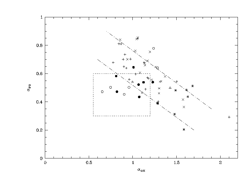
Figure 3 shows the ![]() diagramfor our sample. The different types of objects are represented by
the different symbols explained in the figure caption. The dashed square
represents the limits given by Schachter et al. (1993) for the region occupied
by the XBLs. The dash-dotted lines are the limits for the regions occupied
by XBLs (lower-left) and RBLs (upper-right) according to Padovani &
Giommi (1995).
diagramfor our sample. The different types of objects are represented by
the different symbols explained in the figure caption. The dashed square
represents the limits given by Schachter et al. (1993) for the region occupied
by the XBLs. The dash-dotted lines are the limits for the regions occupied
by XBLs (lower-left) and RBLs (upper-right) according to Padovani &
Giommi (1995).
The most important thing to notice from the diagram is the position of the known BL Lacs and the new ones. The known objects fall in the distinct regions of the diagram described above, as if there were two separated groups, XBLs and RBLs.
Based on this fact, several authors (Garilli et al. 1990; Stocke et
al. 1991) have claimed that the population of BL Lacs is divided into two
groups: XBLs and RBLs. The regions in the ![]() diagram occupied by both groups are displayed in Figure 3. From our diagram
it is clear that there are BL Lacs which ``fill'' the gap between these
two BL Lac classes (see also Nass et al. 1996; Kock et al. 1996). Whereas
the known BL Lacs form two separate groups in the diagram, the RBLs and
the XBLs, the gap disappears if the new BL Lacs from our survey are included.
It is possible that the bimodality is artificially introduced by the properties
of the samples used. For instance, the BL Lacs from the EMSS tend to almost
exclusively populate the XBL-region of the diagram. This can be a consequence
of the follow-up identification programs that have concentrated on objects
inside the square (Schachter et al. 1993; Perlman et al. 1996).
diagram occupied by both groups are displayed in Figure 3. From our diagram
it is clear that there are BL Lacs which ``fill'' the gap between these
two BL Lac classes (see also Nass et al. 1996; Kock et al. 1996). Whereas
the known BL Lacs form two separate groups in the diagram, the RBLs and
the XBLs, the gap disappears if the new BL Lacs from our survey are included.
It is possible that the bimodality is artificially introduced by the properties
of the samples used. For instance, the BL Lacs from the EMSS tend to almost
exclusively populate the XBL-region of the diagram. This can be a consequence
of the follow-up identification programs that have concentrated on objects
inside the square (Schachter et al. 1993; Perlman et al. 1996).
Our data reveal the existence of an intermediate type of BL Lacs. These
objects are located between RBLs and XBLs in the ![]() diagram. Kock et al. (1996), Nass et al. (1996) and more recently Laurent-Muehleisen
et al. (1997) also found several of these BL Lacs in their samples. This
finding has been interpreted as a transition in the broad band properties
from one class of BL Lacs to the other and put some restrictions to the
unification models.
diagram. Kock et al. (1996), Nass et al. (1996) and more recently Laurent-Muehleisen
et al. (1997) also found several of these BL Lacs in their samples. This
finding has been interpreted as a transition in the broad band properties
from one class of BL Lacs to the other and put some restrictions to the
unification models.
For instance, Padovani and Giommi (1995) proposed that RBLs and XBLs
have the same range in orientation angles with respect to the line of sight,
but intrinsically different spectral energy distributions (SEDs) and suggested
that the main difference between XBLs and RBLS is the the frequency at
which the synchrotron break occurs (Different Energy Cutoff scenario).
This model predicts the existence of two separated groups of BL Lacs in
the ![]() diagram.
Padovani and Giommi were able to reproduce the distribution of the EMSS
and the 1 Jy samples accurately in this diagram. However, the existence
of intermediate objects was not taken into account in this model.
diagram.
Padovani and Giommi were able to reproduce the distribution of the EMSS
and the 1 Jy samples accurately in this diagram. However, the existence
of intermediate objects was not taken into account in this model.
On the other hand, in the different viewing angle model, the properties
of the objects depend on the orientation of the jet with respect to the
vieving angle. The RBLs are the objects with smaller angles, where the
stronger radio emission rises more steeply, i.e., the spectral indices
shift toward the upper right corner in the ![]() diagram.
diagram.
If the class of BL Lac is determined only by the orientation, it is
expected a smooth variation of the properties with varying viewing angle
relative to the jet axis. However, there are other properties of BL Lacs
that can not be explained only as a geometrical effect (Sambruna el al.
1996; Heidt & Wagner 1998). Nevertheless, a model based in a varying
viewing angle and the kinetic luminosity of the jet (Georganopoulos &
Marscher, 1998) predicts the continuos distribution of BL Lacs in the ![]() diagram among other properties.
diagram among other properties.
In this way, it is possible to say that the BL Lacs form one group of
objects that was separated in two groups due to selection strategies. This
is also supported by the continuous variation of amplitudes with the spectral
indices.
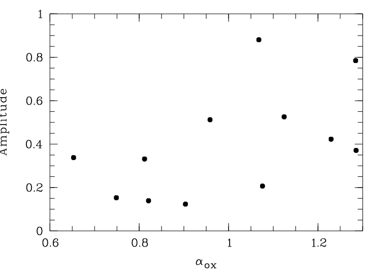
Correlations
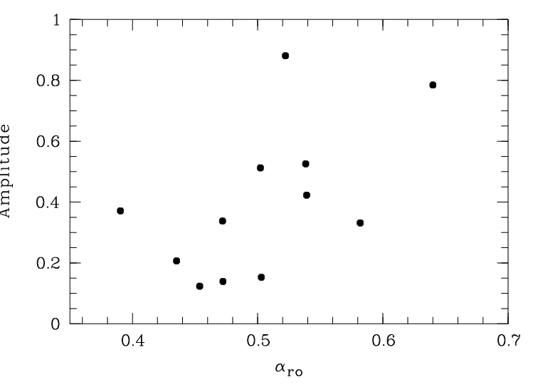
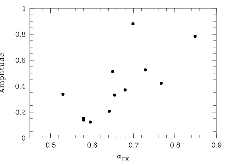
We plotted the amplitude of the light curves versus the spectral indices
of the BL Lacs in order to check if there exist a correlation between the
energy distribution and the variability. We found a dependence of the amplitude
on the three indices, ![]() ,
, ![]() and
and ![]() .
The correlation of amplitude and spectral index is strongest for
.
The correlation of amplitude and spectral index is strongest for ![]() ,
where objects with flatter overall spectrum, from radio to X-ray, show
smaller amplitude in the light curve.
,
where objects with flatter overall spectrum, from radio to X-ray, show
smaller amplitude in the light curve.
For ![]() there
is also a clear correlation whereas for
there
is also a clear correlation whereas for ![]() it is less significant. For this index an inclined upper envelope of the
amplitude-spectral index distribution seems to exist. These correlations
suggest a continuous transition from XBLs to RBLs.
it is less significant. For this index an inclined upper envelope of the
amplitude-spectral index distribution seems to exist. These correlations
suggest a continuous transition from XBLs to RBLs.
It is possible that for some of the objects, with only a couple of runs,
we are not measuring the highest amplitude. Longer time coverage could
improve the determination of the amplitude.
Comparison of Search Techniques
The most common methods employed to select BL Lacs from a sample of X-ray sources are based mainly on the values on the ratios of monochromatic fluxes in the optical, X-ray and radio band.
The ![]() diagram
has proven to be a very useful tool to classify extragalactic objects (Stocke
et al. 1991), especially to discover new BL Lac objects (Schachter et al.
1993). However, for some intermediate BL Lacs it is not the best way to
identify them since a search restricting candidate selection to the XBL
and RBL regions would find XBLs or RBLs. This diagram is very useful, but
needs to be complemented with other properties of the BL Lacs such as polarization
or variability.
diagram
has proven to be a very useful tool to classify extragalactic objects (Stocke
et al. 1991), especially to discover new BL Lac objects (Schachter et al.
1993). However, for some intermediate BL Lacs it is not the best way to
identify them since a search restricting candidate selection to the XBL
and RBL regions would find XBLs or RBLs. This diagram is very useful, but
needs to be complemented with other properties of the BL Lacs such as polarization
or variability.
Stocke et al. (1985) also proposed to use the log(fx/fv)(=
logfx
+ V/2.5 + 5.37) to discriminate BL Lacs from other X-ray emitters
since BL Lacs are those AGN which show the highest values of the fluxes
ratio (corresponding to the lowest ![]() ).
Selecting candidates with high log(fx/fv)
has the advantage that it is independent of radio observations. Nass et
al. (1996) found that 40% of the objects showing log(fx/fv)
> 1.3were confirmed BL Lacs via spectroscopy.
).
Selecting candidates with high log(fx/fv)
has the advantage that it is independent of radio observations. Nass et
al. (1996) found that 40% of the objects showing log(fx/fv)
> 1.3were confirmed BL Lacs via spectroscopy.
We computed the log(fx/fv)
ratios for the objects in our sample. The histogram in Figure 5 shows the
distribution of the whole sample of radio sources. The distribution of
the BL Lac objects is represented by the shaded area.
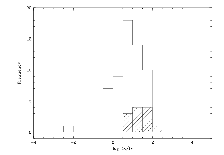
It can be seen from the figure that for those objects with log(fx/fv)
> 1.5, aproximately 50% are, in fact, BL Lacs. However, worth noticing
is that the rest or 50% of the BL Lacs have log(fx/fv)
< 1.5. These objects would be ignored by using exclusively this criteria.
This situation is similar as in the case of the ![]() diagram. All of these objects correspond to the intermediate population
discussed in the
diagram. All of these objects correspond to the intermediate population
discussed in the ![]() diagram of our sample.
diagram of our sample.
Summarizing, these two techniques seem to be highly efficient to pre-identify
BL Lacs from large samples. However, if the goal is to identify all the
BL Lacs in a sample, in order to test unification models, it is better
to used complementary criteria.
Conclusions
We tested the optical variability as an extra tool to identified BL Lacs in a sample of X-ray sources. We demonstrated that variability studies are helpful to identify BL Lac objects.
For the identification we also used as another tool their distinctive
X-ray/optical/radio colors (![]() diagram). However, an important result is that part of the BL Lacs in our
sample show properties intermediate between RBLs and XBLs, which could
make their identification, based only in their position in the diagram,
more difficult.
diagram). However, an important result is that part of the BL Lacs in our
sample show properties intermediate between RBLs and XBLs, which could
make their identification, based only in their position in the diagram,
more difficult.
It seems that the optical variability is related with the broad-band
properties. We found a correlation between the amplitude and the spectral
indices. In addition, we have found that the timescales of the variations
are shorter for RBLs than for XBLs. This can be seen from Table 2 where
the objects with smaller ![]() are suspicious to be non-variable on the timescales of days, while the
rest are clearly variable in this timescale.
are suspicious to be non-variable on the timescales of days, while the
rest are clearly variable in this timescale.
The correlations in addition to the existence of intermediate objects, favor the idea that BL Lacs form only one population of objects that has been separated in two subgroups due to the strategies followed for preselection of candidates.
The existence of intermediate values in the spectral indices exhibited by BL Lacs in our sample has important implications for unification models. A recent model, based in the orientation angle of the relativistic jet and the kinetic luminosity of the jet, predicts the existence of the intermediate objects.
The techniques discussed in the last section (logfx/fv
and ![]() diagram)
seem to be highly efficient to pre-identify BL Lacs from large samples.
However, as we discussed, not all the objects are picked with this technique.
There are several BL Lacs that could have been missed, and if what we desire
is to identify all the BL Lacs in a sample (in order to achieve completeness),
the candidates cannot be chosen only based in their SEDs. It would be better
to make use of as many properties as possible to recognize these objects.
diagram)
seem to be highly efficient to pre-identify BL Lacs from large samples.
However, as we discussed, not all the objects are picked with this technique.
There are several BL Lacs that could have been missed, and if what we desire
is to identify all the BL Lacs in a sample (in order to achieve completeness),
the candidates cannot be chosen only based in their SEDs. It would be better
to make use of as many properties as possible to recognize these objects.