Globular Cluster Luminosity Function Analysis

Pablo G. Ostrov

Facultad de Ciencias Astronómicas y Geofísicas, Paseo del Bosque S/N (1900) La Plata, Argentina

ostrov@fcaglp.fcaglp.unlp.edu.ar

http://www.fcaglp.unlp.edu.ar/~ostrov/

INTRODUCTION.

One of the most common problems of astronomical work is that of distance determination. Astronomers wish to find objects bright enough to be useful as standard candles.

Undoubtedly, globular clusters are bright enough to be considered potentially interesting objects for distance determination. The obstacle arising from the broad range that they span in luminosity brightness can be avoided by observing samples of many of them, and then using the globular cluster luminosity function (GCLF) as a standard candle.

Harris, Allwright, Pritchet and van den Bergh (1991) analyzed observations of three Virgo giant ellipticals, founding no noticeable differences between their GCLFs.

In virtue of the progressive advance of astronomical technology, it has been feasible to study globular cluster systems of an increasing sample of galaxies. It is now possible to begin to investigate the second order differences between GCLFs, and its relations with their environments and metallicities.

MOTIVATION

From a practical point of view, the determination of GCLF parameters presents several problems:

1.- One frequently observes the bright half of the luminosity distribution, and losses an usually significant fraction of the faint half.

2.- The sample of globulars is unavoidably contaminated by interlopers, and this contamination must be removed by means of some statistical consideration. Only in several nearby galaxies is feasible, with space telescope observations, to resolve the globulars and thus to distinguish them from foreground stars and unresolved background objects.

The aim of this work is to investigate the credibility of GCLF parameter determinations, and how incompleteness and contamination affect the results. It is needed to answer some basic questions, as how many magnitudes deeper than the turn-over it is required to observe to obtain reliable parameter estimates, and how many clusters should have a sample to be suitable for GCLF analysis.

NUMERICAL EXPERIMENTS

In order to answer the above formulated questions, series of observed luminosity distribution models were generated. These models were analyzed by means of a maximum likelihood method (Secker & Harris, 1993) that allows to obtain simultaneously the peak of the luminosity distribution m₀ and the dispersion $\sigma$. A previous work was performed by Hanes & Whittaker (1987), addressed specifically to GCSs at distances such as the Virgo Cluster.

PARAMETERS OF MODELS

GCLF: Two types of distributions were generated

$${\rm gaussian:} \qquad \qquad N(m) \sim A \exp \left\{{- {(m-m_{0})^{2}\over 2 \sigma ^{2}}}\right\}$$

$${\rm and}~~t_{5} \qquad \qquad N(m) \sim A \left\{{1 + {(m-m_{0})^{2}\over 5 \sigma ^{2}}}\right\}^{-3}$$

Completeness: It was modeled by means of a Pritchet function

$$f_c={1\over 2}\left\{{1-{\alpha (m-m_{lim})\over \sqrt{1+\alpha^{2}(m-m_{lim})^{2}}}}\right\}$$

where m_lim stands for the $50 \%$ completeness level magnitude and the shape parameter $\alpha$ was chosen to be equal to 2.4.

N_gc: Regarding the total number of globular clusters N_gc, three series of models were generated with 400, 2000 and 10000 globulars each one.

m_cut: It represents the faintest magnitude at which the data are considered useful. Surpassing this limit, all data are removed and the completeness factor is set to zero. Series of models with m_cut equivalent to $40\%, 60\%$ and $80\%$ of completeness were generated.

Background: The background population was modeled by means of the distribution

$$\log n = 0.445 m_{0} + c$$

The slope was obtained by least squares fitting to a real background data sample and the density of background objects was chosen according to realistic cases. For each model a separate ``background data set'' was generated to simulate the ``background field'' used for background contamination correction.

m₀: Samples with luminosity function peak at 23.25, 23.75, 24.25 and 24.75 were generated. These corresponds to distances ranging from 16 Mpc to 40 Mpc approximately.

Initial conditions: Being the analysis based on a maximum likelihood method, the solution converges to a local maximum. For this reason, the influence of the starting guesses on the results were also investigated.

A total of 1000 data sets were generated for each model, therefore the following results comprise the analysis of more than one million of fittings.

RESULTS

1.- Choice of m_cut:

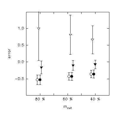
The choice of m_cut is not a critical one. In the cases in which some systematic behavior of the errors is noticeable, the better results are obtained for the faintest m_cut.

Figure 1 shows an example of the dependence of errors in m₀ fittings for different value of m_cut. Circles correspond to gaussian models and triangles to t₅ models. Hollow symbols stand for gaussian fittings and filled symbols stand for t₅ fittings.

2.- In which cases the estimates for $\sigma$ are reliable?

The accurate determination of $\sigma$ is feasible only if the peak of the luminosity function has been surpassed by, at least, two magnitudes. Even in such cases, errors of $0.1 \sim 0.2$ occur if the contamination of the sample is meaningful.

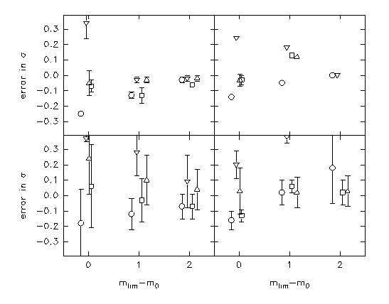
Figure 2 shows the errors in the adjustment of $\sigma$. Top panels correspond to a very low contamination case, m₀=23.35 and N_gc=10000. The results displayed in the bottom panels correspond to a high contamination case, with m₀=24.75 and N_gc=400. This is equivalent to observed counts of N^obs_gc=365 and N^obs_bkg=300 for m_lim =m₀+2, and to N^obs_gc=300 and N^obs_bkg=100 objects for m_lim =m₀+1. Left and right panels concern respectively to gaussian and t₅ distributions. Different symbols stand for distinct starting guesses.

3.- And where is the turn-over?

It is needed to surpass clearly the turn-over to obtain reliable estimates of m₀. If m₀=m_lim , the resulting fitted parameters are affected by significant systematic errors. If m₀-m_lim =-1, then the errors in m₀ estimates tend just to -1, that is, it is not possible to distinguish between the true turn-over and the drop of completeness.

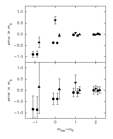
Figure 3 displays the errors in the determination of m₀. Top and bottom panels show respectively the above mentioned cases of low and high contamination. Circles and inverted triangles represent gaussian fittings performed on gaussian and t₅ distributions respectively. Squares and triangles indicate t₅ fittings to gaussian and t₅ distributions.

REFERENCES

Hanes & Whittaker, 1987, AJ, 94, 906

Harris, Allwright, Pritchet & van den Bergh, 1991, ApJS, 76, 115

Secker & Harris, 1993, AJ, 105, 1358